

![]()

Positive-unlabeled learning with Python.
Website: https://pulearn.github.io/pulearn/
Documentation: https://pulearn.github.io/pulearn/doc/pulearn/
from pulearn import ElkanotoPuClassifier
from sklearn.svm import SVC
svc = SVC(C=10, kernel='rbf', gamma=0.4, probability=True)
pu_estimator = ElkanotoPuClassifier(estimator=svc, hold_out_ratio=0.2)
pu_estimator.fit(X, y)
Contents
- 1 Documentation
- 2 Installation
- 3 Extending
pulearn - 4 Implemented Classifiers
- 5 Evaluation Metrics
- 6 Model Selection
- 7 Examples
- 8 Contributing
- 9 License
- 10 Credits
This is the repository for the pulearn package. The readme file is aimed at helping contributors to the project.
To learn more about how to use pulearn, either visit pulearn's homepage or read the documentation at <https://pulearn.github.io/pulearn/doc/pulearn/>`_.
Install pulearn with:
pip install pulearnNew learner work now goes through a small registry and contributor scaffold:
pulearn.get_algorithm_registry()exposes discoverable metadata for the built-in learners.doc/new_algorithm_checklist.mddefines the required contributor steps.doc/templates/new_algorithm_doc_stub.mdis the docs page starting point.tests/templates/test_new_algorithm_template.py.tmplandtests/templates/test_api_contract_template.py.tmplprovide regression and shared API contract scaffolds.benchmarks/templates/benchmark_entry_template.py.tmplis the benchmark stub until the benchmark harness lands in the dedicated roadmap milestone.pulearn.get_scaffold_templates()resolves those scaffold files only from a repository checkout and fails clearly when they are unavailable.
At minimum, every new learner should register metadata, add focused tests,
run the shared API contract checks when it inherits from
BasePUClassifier, and add docs plus a benchmark placeholder in the same
PR.
Scikit-Learn wrappers for both the methods mentioned in the paper by Elkan and Noto, "Learning classifiers from only positive and unlabeled data" (published in Proceeding of the 14th ACM SIGKDD international conference on Knowledge discovery and data mining, ACM, 2008).
These wrap the Python code from a fork by AdityaAS (with implementation to both methods) to the original repository by Alexandre Drouin implementing one of the methods.
PU labels are normalized to a canonical internal representation
(1 = labeled positive, 0 = unlabeled). Accepted input conventions
include {1, -1}, {1, 0}, and {True, False}.
Use pulearn.normalize_pu_labels(...) to normalize labels immediately at
ingest or estimator/metric boundaries.
To use the classic (unweighted) method, use the ElkanotoPuClassifier class:
from pulearn import ElkanotoPuClassifier
from sklearn.svm import SVC
svc = SVC(C=10, kernel='rbf', gamma=0.4, probability=True)
pu_estimator = ElkanotoPuClassifier(estimator=svc, hold_out_ratio=0.2)
pu_estimator.fit(X, y)To use the weighted method, use the WeightedElkanotoPuClassifier class:
from pulearn import WeightedElkanotoPuClassifier
from sklearn.svm import SVC
svc = SVC(C=10, kernel='rbf', gamma=0.4, probability=True)
pu_estimator = WeightedElkanotoPuClassifier(
    estimator=svc, labeled=10, unlabeled=20, hold_out_ratio=0.2)
pu_estimator.fit(X, y)
See the original paper for details on how the labeled and unlabeled quantities are used to weigh training examples and affect the learning process: https://cseweb.ucsd.edu/~elkan/posonly.pdf.
Based on the paper A bagging SVM to learn from positive and unlabeled examples (2013) by Mordelet and Vert. The implementation is by Roy Wright (roywright on GitHub), and can be found in his repository.
Accepted PU label conventions match the package-wide contract:
1/True for labeled positives and 0/-1/False for
unlabeled examples.
from pulearn import BaggingPuClassifier
from sklearn.svm import SVC
svc = SVC(C=10, kernel='rbf', gamma=0.4, probability=True)
pu_estimator = BaggingPuClassifier(
    estimator=svc, n_estimators=15)
pu_estimator.fit(X, y)Implements the nnPU algorithm from
Kiryo et al. (NeurIPS 2017).
Trains a linear classifier using a non-negative risk estimator that prevents
overfitting to positive examples. Supports both nnPU (non-negative, default)
and uPU (unbiased) modes. The prior probability of the positive class must
be provided.
from pulearn import NNPUClassifier

clf = NNPUClassifier(prior=0.3, max_iter=1000, learning_rate=0.01)
clf.fit(X_train, y_pu)  # y_pu: 1 = labeled positive, 0 or -1 = unlabeled
labels = clf.predict(X_test)
Use nnpu=False to switch to unbiased PU (uPU) mode, which does not apply
the non-negative correction and may be better suited to datasets where the
labeled-positive set is large and well-calibrated.
Bayesian classifiers for PU learning based on the MIT-licensed Bayesian Classifiers for PU Learning project by Chengning Zhang.
All four classifiers accept the same package-wide PU label conventions:
{1, 0}, {1, -1}, and {True, False}. Continuous features are
automatically discretized into equal-width bins.
The simplest Bayesian PU classifier. Class-conditional distributions
P(x|y=1) and P(x|y=0) are estimated from the labeled positives
and the unlabeled set (treated as approximate negatives) respectively, with
Laplace smoothing controlled by alpha.
from pulearn import PositiveNaiveBayesClassifier

clf = PositiveNaiveBayesClassifier(alpha=1.0, n_bins=10)
clf.fit(X_train, y_pu)           # y_pu: 1 = labeled positive, 0 = unlabeled
proba = clf.predict_proba(X_test)  # shape (n_samples, 2): [P(y=0|x), P(y=1|x)]
labels = clf.predict(X_test)Extends PNB by weighting each feature's log-likelihood contribution by its empirical mutual information with the PU label. Features that are more informative receive higher weights; all weights are non-negative and sum to 1.
from pulearn import WeightedNaiveBayesClassifier

clf = WeightedNaiveBayesClassifier(alpha=1.0, n_bins=10)
clf.fit(X_train, y_pu)
print(clf.feature_weights_)      # normalized MI weight per feature (sums to 1)
proba = clf.predict_proba(X_test)Extends PNB by replacing the naive feature-independence assumption with a tree structure learned via the Chow-Liu algorithm. Pairwise conditional mutual information I(X_i; X_j \mid S) is computed for all feature pairs, and a maximum spanning tree is built with Prim's algorithm. Each non-root feature depends on exactly one parent feature in addition to the class label.
from pulearn import PositiveTANClassifier

clf = PositiveTANClassifier(alpha=1.0, n_bins=10)
clf.fit(X_train, y_pu)
print(clf.tan_parents_)          # parent index per feature; -1 for the root
proba = clf.predict_proba(X_test)Combines PTAN's tree structure with WNB's per-feature MI weighting.
from pulearn import WeightedTANClassifier

clf = WeightedTANClassifier(alpha=1.0, n_bins=10)
clf.fit(X_train, y_pu)
print(clf.feature_weights_)      # normalized MI weight per feature
print(clf.tan_parents_)          # learned tree structure
proba = clf.predict_proba(X_test)
A complete end-to-end example on the Wisconsin breast cancer dataset can be
found in the examples directory:
python examples/BayesianPULearnersExample.pypulearn.priors now exposes a small, unified class-prior estimation API
for SCAR workflows:
LabelFrequencyPriorEstimatorreturns the observed labeled-positive rate as a naive lower bound for \pi.HistogramMatchPriorEstimatorfits a probabilistic scorer and matches labeled-positive vs. unlabeled score histograms.ScarEMPriorEstimatorruns a soft-label EM refinement loop over latent positives in the unlabeled pool.
All three implement fit(X, y) and estimate(X, y) and return a
PriorEstimateResult with the estimated prior, sample counts, and
method-specific metadata.
from pulearn import (
    HistogramMatchPriorEstimator,
    LabelFrequencyPriorEstimator,
    ScarEMPriorEstimator,
)

baseline = LabelFrequencyPriorEstimator().estimate(X_train, y_pu)
histogram = HistogramMatchPriorEstimator().estimate(X_train, y_pu)
scar_em = ScarEMPriorEstimator().estimate(X_train, y_pu)

print(baseline.pi, histogram.pi, scar_em.pi)
print(scar_em.metadata["c_estimate"])
Bootstrap confidence intervals are available when you need uncertainty estimates or reproducible sensitivity checks:
estimator = ScarEMPriorEstimator().fit(X_train, y_pu)
result = estimator.bootstrap(
    X_train,
    y_pu,
    n_resamples=200,
    confidence_level=0.95,
    random_state=7,
)

print(result.confidence_interval.lower, result.confidence_interval.upper)
Diagnostics helpers can summarize estimator stability across a parameter sweep and optionally drive sensitivity plots:
from pulearn import (
    HistogramMatchPriorEstimator,
    diagnose_prior_estimator,
)

diagnostics = diagnose_prior_estimator(
    HistogramMatchPriorEstimator(),
    X_train,
    y_pu,
    parameter_grid={"n_bins": [8, 12, 20], "smoothing": [0.5, 1.0]},
)

print(diagnostics.unstable, diagnostics.warnings)
print(diagnostics.range_pi, diagnostics.std_pi)

# Optional: requires matplotlib
# from pulearn import plot_prior_sensitivity
# plot_prior_sensitivity(diagnostics)
If pi is uncertain, you can sweep corrected metrics across a plausible prior range and inspect best/worst-case behavior:
from pulearn import analyze_prior_sensitivity

sensitivity = analyze_prior_sensitivity(
    y_pu,
    y_pred=y_pred,
    y_score=y_score,
    metrics=["pu_precision", "pu_roc_auc"],
    pi_min=0.2,
    pi_max=0.5,
    num=7,
)

print(sensitivity.as_rows())
print(sensitivity.summaries["pu_precision"].best_pi)pulearn.propensity provides first-class estimators for the SCAR labeling
propensity c = P(s=1 \mid y=1):
MeanPositivePropensityEstimatormatches the classic Elkan-Noto mean-on-positives estimate.TrimmedMeanPropensityEstimatorreduces sensitivity to a few badly calibrated labeled positives.MedianPositivePropensityEstimatorandQuantilePositivePropensityEstimatorgive conservative alternatives when positive scores are noisy or skewed.CrossValidatedPropensityEstimatoruses out-of-fold probabilities from a probabilistic sklearn estimator to reduce optimistic bias.
All score-based estimators implement fit(y_pu, s_proba=...) and
estimate(y_pu, s_proba=...). The cross-validated estimator uses the same
API but takes X=... plus a base estimator.
from sklearn.linear_model import LogisticRegression

from pulearn import (
    CrossValidatedPropensityEstimator,
    MeanPositivePropensityEstimator,
    MedianPositivePropensityEstimator,
    QuantilePositivePropensityEstimator,
    TrimmedMeanPropensityEstimator,
)

mean_c = MeanPositivePropensityEstimator().estimate(y_pu, s_proba=y_score)
trimmed_c = TrimmedMeanPropensityEstimator(trim_fraction=0.1).estimate(
    y_pu,
    s_proba=y_score,
)
median_c = MedianPositivePropensityEstimator().estimate(
    y_pu,
    s_proba=y_score,
)
quantile_c = QuantilePositivePropensityEstimator(quantile=0.25).estimate(
    y_pu,
    s_proba=y_score,
)
cv_c = CrossValidatedPropensityEstimator(
    estimator=LogisticRegression(max_iter=1000),
    cv=5,
    random_state=7,
).estimate(y_pu, X=X_train)

print(mean_c.c, trimmed_c.c, median_c.c, quantile_c.c, cv_c.c)
print(cv_c.metadata["fold_estimates"])
pulearn.metrics.estimate_label_frequency_c(...) now delegates to the same
mean estimator and therefore expects probability-like scores in [0, 1].
Bootstrap confidence intervals are available for propensity estimators when you need uncertainty estimates or a warning that the labeling mechanism looks unstable under resampling:
estimator = TrimmedMeanPropensityEstimator(trim_fraction=0.1).fit(
    y_pu,
    s_proba=y_score,
)
result = estimator.bootstrap(
    y_pu,
    s_proba=y_score,
    n_resamples=200,
    confidence_level=0.95,
    random_state=7,
)

print(result.c)
print(result.confidence_interval.lower)
print(result.confidence_interval.upper)
print(result.confidence_interval.warning_flags)
Instability warnings flag repeated fit failures, unusually high resample
variance, large coefficient of variation, or inconsistent cross-validation
fold estimates. Treat those warnings as a signal to inspect calibration,
selection bias, or mislabeled positives before using c downstream.
You can also compare labeled positives against the highest-scoring unlabeled pool to look for likely SCAR violations:
from pulearn import scar_sanity_check

scar_check = scar_sanity_check(
    y_pu,
    s_proba=y_score,
    X=X_train,
    candidate_quantile=0.9,
    random_state=7,
)

print(scar_check.group_membership_auc)
print(scar_check.max_abs_smd)
print(scar_check.warnings)
Warnings such as group_separable or max_feature_shift mean the
high-scoring unlabeled pool looks materially different from labeled
positives, which is a practical sign that SCAR may not hold closely enough
for naive propensity correction.
pulearn now exposes a minimal experimental interface for SAR-style
selection models. The scope is intentionally narrow: you can plug in a
propensity model and derive inverse-propensity weights, but this does not
yet implement full SAR learners or SAR-corrected metrics.
from sklearn.linear_model import LogisticRegression

from pulearn import (
    ExperimentalSarHook,
    compute_inverse_propensity_weights,
    predict_sar_propensity,
)

propensity_model = LogisticRegression(max_iter=1000).fit(X_train, s_train)

sar_scores = predict_sar_propensity(propensity_model, X_test)
sar_weights = compute_inverse_propensity_weights(
    sar_scores,
    clip_min=0.05,
    clip_max=1.0,
    normalize=True,
)

hook = ExperimentalSarHook(propensity_model)
hook_result = hook.inverse_propensity_weights(X_test, normalize=True)

print(hook_result.weights[:5])
print(hook_result.metadata["propensity_model"])
These helpers emit experimental warnings on purpose. Treat them as plumbing for custom SAR research code rather than a stable high-level workflow. Always inspect the clipped counts and weight magnitudes before using them downstream.
Standard binary classification metrics (precision, recall, F1) are systematically
biased in PU settings: a trivial classifier that predicts positive for every sample
achieves recall = 1.0 with no penalty for false positives in the unlabeled pool.
pulearn.metrics provides unbiased estimators that cover the full evaluation
lifecycle under the SCAR (Selected Completely At Random) assumption.
Note
All PU metrics assume SCAR as their baseline. If selection bias is present (SAR / SNAR settings) you will need inverse propensity weighting on top of these estimators.
Before computing confusion-matrix metrics you must map the model's observed output P(s=1|x) to the calibrated posterior P(y=1|x).
from pulearn.metrics import estimate_label_frequency_c, calibrate_posterior_p_y1

# 1. Estimate the propensity score c = P(s=1 | y=1)
c_hat = estimate_label_frequency_c(y_pu, s_proba)

# 2. Calibrate: P(y=1|x) ≈ P(s=1|x) / c
p_y1 = calibrate_posterior_p_y1(s_proba, c_hat)
estimate_label_frequency_c implements the Elkan-Noto estimator
\hat{c} \approx \mathbb{E}[P(s=1|x) \mid s=1].
calibrate_posterior_p_y1 clips P(s=1|x) / \hat{c} to [0, 1].
These metrics reconstruct the confusion matrix from calibrated posteriors rather than treating unlabeled data as confirmed negatives.
from pulearn.metrics import (
    pu_recall_score,
    pu_precision_score,
    pu_f1_score,
    pu_specificity_score,
)

# Recall on labeled positives (no class prior needed)
rec  = pu_recall_score(y_pu, y_pred)

# Unbiased precision and F1 require the class prior π
prec = pu_precision_score(y_pu, y_pred, pi=0.3)
f1   = pu_f1_score(y_pu, y_pred, pi=0.3)

# Expected specificity — returns 0.0 for any all-positive classifier
spec = pu_specificity_score(y_pu, y_score)
pu_specificity_score is particularly useful as a sanity-check guard: a
degenerate classifier that assigns every sample to the positive class obtains
\text{spec} = 0, immediately flagging the model as trivial.
Two AUC-based metrics correct for the absence of ground-truth negatives.
from pulearn.metrics import pu_roc_auc_score, pu_average_precision_score

# Sakai (2018) adjustment: AUC_pn = (AUC_pu − 0.5π) / (1 − π)
auc = pu_roc_auc_score(y_pu, y_score, pi=0.3)

# Area Under Lift: AUL = 0.5π + (1 − π) · AUC_pu
aul = pu_average_precision_score(y_pu, y_score, pi=0.3)
pu_roc_auc_score maps the biased AUC_{pu} (computed against PU labels)
to an unbiased estimator of the true positive-vs-negative AUC.
pu_average_precision_score returns the Area Under Lift (AUL), which is more
robust to severe class imbalance.
For flexible models such as deep networks, raw risk estimators are suitable for early stopping and model selection in lieu of black-box accuracy metrics.
from pulearn.metrics import pu_unbiased_risk, pu_non_negative_risk

# uPU: pi * R_p+ + R_u- - pi * R_p-  (du Plessis et al., 2015)
risk_upu  = pu_unbiased_risk(y_pu, y_score, pi=0.3)

# nnPU: clamps negative component to zero to prevent over-fitting
#        (Kiryo et al., 2017)
risk_nnpu = pu_non_negative_risk(y_pu, y_score, pi=0.3)
Both functions accept a loss argument (currently "logistic").
Two utility functions help detect why a model may be performing poorly.
from pulearn.metrics import pu_distribution_diagnostics, homogeneity_metrics

# KL divergence between labeled and unlabeled score distributions
# Near-zero divergence → model cannot separate positives from unlabeled
diag = pu_distribution_diagnostics(y_pu, y_score)
print(diag["kl_divergence"])

# STD and IQR of predicted-negative scores
# Low STD/IQR → model may be over-relying on trivial features
hom_metrics = homogeneity_metrics(y_pu, y_score)
print(hom_metrics["std"], hom_metrics["iqr"])make_pu_scorer wraps any PU metric as a make_scorer-compatible callable,
enabling direct use with GridSearchCV and RandomizedSearchCV.
from sklearn.model_selection import GridSearchCV
from pulearn.metrics import make_pu_scorer

scorer = make_pu_scorer("pu_f1", pi=0.3)

gs = GridSearchCV(estimator, param_grid, scoring=scorer)
gs.fit(X_train, y_pu_train)
Supported metric names for make_pu_scorer:
"lee_liu" |
Lee & Liu score (no pi required) |
"pu_recall" |
PU recall (no pi required) |
"pu_precision" |
Unbiased PU precision |
"pu_f1" |
Unbiased PU F1 |
"pu_specificity" |
Expected specificity |
"pu_roc_auc" |
Adjusted ROC-AUC (Sakai 2018) |
"pu_average_precision" |
Area Under Lift (AUL) |
"pu_unbiased_risk" |
uPU risk (lower is better) |
"pu_non_negative_risk" |
nnPU risk (lower is better) |
Risk metrics are wrapped with greater_is_better=False so that
GridSearchCV correctly minimises them.
An end-to-end demo comparing naive F1 inflation vs. corrected metrics on
synthetic SCAR data can be found in the examples directory:
python examples/PUMetricsEvaluationExample.pypulearn.model_selection provides PU-aware splitting utilities that ensure
labeled positive samples are preserved across all folds and splits. Under the
SCAR assumption, stratifying by the binary PU label (labeled=1 vs. unlabeled=0)
is a valid and practical proxy for preserving the labeled-positive rate.
Wraps sklearn.model_selection.StratifiedKFold and stratifies by the
PU label so that each fold contains roughly the same fraction of labeled
positive samples as the full dataset.
from sklearn.svm import SVC
from pulearn import PUStratifiedKFold

estimator = SVC()
scores = []
cv = PUStratifiedKFold(n_splits=5, shuffle=True, random_state=0)
for train_idx, test_idx in cv.split(X, y_pu):
    estimator.fit(X[train_idx], y_pu[train_idx])
scores.append(estimator.score(X[test_idx], y_pu[test_idx]))A higher-level PU cross-validator compatible with
sklearn.model_selection.cross_validate and
sklearn.model_selection.GridSearchCV. Emits an actionable
UserWarning when the labeled-positive count is smaller than n_splits
and falls back to plain sklearn.model_selection.KFold in that case.
from sklearn.model_selection import cross_validate
from pulearn import PUCrossValidator

cv = PUCrossValidator(n_splits=5, shuffle=True, random_state=0)
results = cross_validate(estimator, X, y_pu, cv=cv, scoring="f1")Stratified train/test split that preserves the PU label distribution and validates that the resulting training set always contains at least one labeled positive.
from pulearn import pu_train_test_split

X_train, X_test, y_train, y_test = pu_train_test_split(
    X, y_pu, test_size=0.2, random_state=42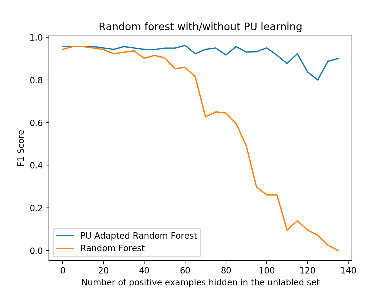
)A nice code example of the classic Elkan-Noto classifier used for classification on the Wisconsin breast cancer dataset , comparing it to a regular random forest classifier, can be found in the examples directory.
To run it, clone the repository, and run the following command from the root of the repository, with a python environment where pulearn is installed:
python examples/BreastCancerElkanotoExample.pyYou should see a nice plot like the one below, comparing the F1 score of the PU learner versus a naive learner, demonstrating how PU learning becomes more effective - or worthwhile - the more positive examples are "hidden" from the training set.
Package author and current maintainer is Shay Palachy (shay.palachy@gmail.com); You are more than welcome to approach him for help. Contributions are very welcomed, especially since this package is very much in its infancy and many other PU Learning methods can be added.
Clone:
git clone git@github.com:pulearn/pulearn.gitInstall in development mode with test dependencies:
cd pulearn
pip install --only-binary=all numpy pandas scikit-learn
pip install -e . -r tests/requirements.txtTo run the tests, use:
python -m pytestpytest is configured in pyproject.toml under [tool.pytest.ini_options].
pulearn targets 100% test coverage. Codecov automatically reports coverage
changes on each PR; pull requests that reduce coverage will not be reviewed
until that is addressed.
Tests live under the tests directory. Each module has a dedicated test file
(prefixed test_) containing individual test functions. Please keep test
cases focused and separate so failures are easy to locate. Thank you! :)
pulearn code is formatted and linted with ruff.
Formatting and lint checks run automatically on every pull request via
GitHub Actions.
To check your changes locally, run:
ruff format .
ruff check . --fix
Pull requests that introduce ruff violations will be flagged by CI.
This project follows the numpy docstring conventions. When documenting code you add to this project, please follow these conventions.
User-facing narrative documentation lives in
src/pulearn/documentation.md (included verbatim in the generated API
docs) and in this README.rst. The docs site is built with
pdoc3; see doc/build.sh and doc/README.md for instructions.
This package is released as open-source software under the BSD 3-clause license. See LICENSE_NOTICE.md for the different copyright holders of different parts of the code.
Implementations code by:
- Elkan & Noto - Alexandre Drouin and AditraAS.
- Bagging PU Classifier - Roy Wright.
- Bayesian PU Classifiers (PNB, WNB, PTAN, WTAN) - ported from Bayesian Classifiers for PU Learning by Chengning Zhang (MIT License).
Packaging, testing and documentation by Shay Palachy.
Fixes and feature contributions by: