REANA example - LHCb Run 2 B+/- -> J/psi K+/- analysis

About

This REANA reproducible analysis example demonstrates how to work with LHCb collision ntuples produced by the LHCb Ntupling Service. The example studies the B+/- -> J/psi K+/- decay channel and demonstrates plotting of the B+/- meson candidate mass and J/psi candidate mass using ROOT RDataFrame.

Analysis structure

Making a research data analysis reproducible basically means to provide "runnable recipes" addressing (1) where is the input data, (2) what software was used to analyse the data, (3) which computing environments were used to run the software and (4) which computational workflow steps were taken to run the analysis. This will permit to instantiate the analysis on the computational cloud and run the analysis to obtain (5) output results.

1. Input data

The analysis uses LHCb Run 2 collision data ntuples from the CERN Open Data portal, accessed live via XRootD from CERN EOS public storage:

• root://eospublic.cern.ch//eos/opendata/lhcb/CollisionNtuples/OPENDATA.LHCB.EBYF.C7OY/outputs/real-production/00334560_00000001_1.dvntuple.root
• root://eospublic.cern.ch//eos/opendata/lhcb/CollisionNtuples/OPENDATA.LHCB.EBYF.C7OY/outputs/real-production/00334560_00000002_1.dvntuple.root
• root://eospublic.cern.ch//eos/opendata/lhcb/CollisionNtuples/OPENDATA.LHCB.EBYF.C7OY/outputs/real-production/00334564_00000001_1.dvntuple.root
• root://eospublic.cern.ch//eos/opendata/lhcb/CollisionNtuples/OPENDATA.LHCB.EBYF.C7OY/outputs/real-production/00334565_00000001_1.dvntuple.root
• root://eospublic.cern.ch//eos/opendata/lhcb/CollisionNtuples/OPENDATA.LHCB.EBYF.C7OY/outputs/real-production/00334566_00000001_1.dvntuple.root

The ntuples contain reconstructed B+/- -> J/psi K+/- decay candidates from the Btree/DecayTree tree.

2. Analysis code

The analysis consists of a single Python script analyse.py that uses ROOT's RDataFrame to read the collision ntuples and produces two histograms:

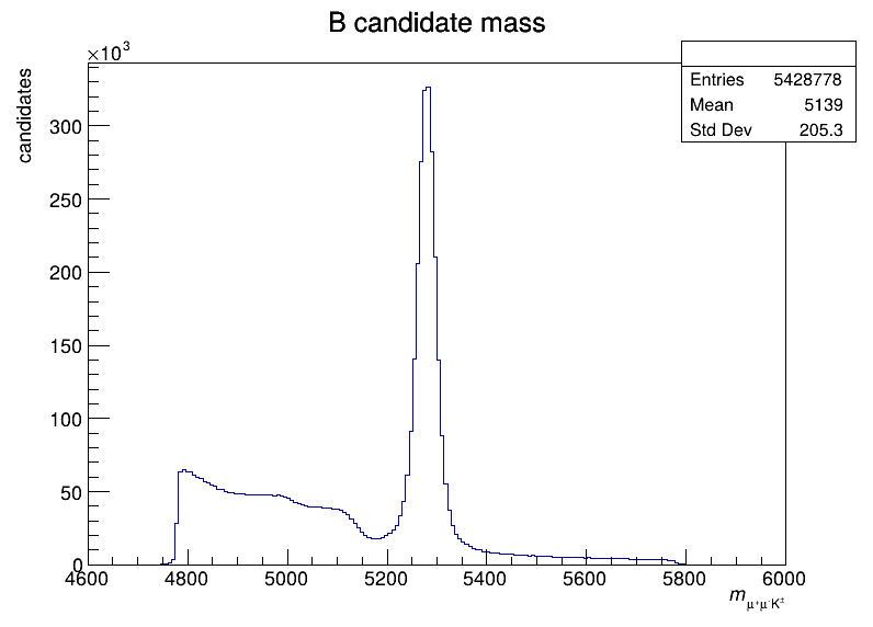
• B+/- meson candidate mass distribution (200 bins, 4600-6000 MeV/c^2)
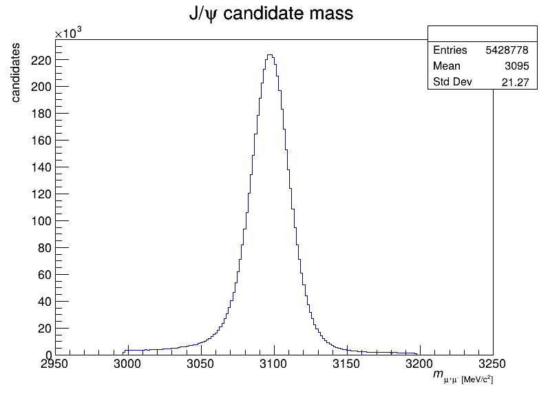
• J/psi candidate mass distribution (200 bins, 2950-3250 MeV/c^2)

3. Compute environment

In order to be able to rerun the analysis even several years in the future, we need to "encapsulate the current compute environment", for example to freeze the ROOT version our analysis is using. We shall achieve this by preparing a Docker container image for our analysis steps.

This analysis example runs within the ROOT6 analysis framework. The computing environment can be therefore easily encapsulated by using the upstream reana-env-root6 base image. We shall use ROOT version 6.38.00. Since our analysis script analyse.py can be uploaded and mounted into the running container at runtime, there is no need to build a new container image specially dedicated to our analysis.

4. Analysis workflow

The analysis workflow is simple and consists of a single step:

              START
               |
               |
               V
+-------------------------------+
| (1) analyse collision ntuples |
|                               |
|    $ python3 analyse.py       |
+-------------------------------+
               |
               | bmass.png
               | jpsimass.png
               V
              STOP

We are using the Snakemake workflow specification (see Snakefile).

5. Output results

The example produces two plots:

The B+/- meson candidate mass distribution:

The J/psi candidate mass distribution:

Running the example on REANA cloud

There are two ways to execute this analysis example on REANA.

If you would like to simply launch this analysis example on the REANA instance at CERN and inspect its results using the web interface, please click on the following badge:

If you would like a step-by-step guide on how to use the REANA command-line client to launch this analysis example, please read on.

We start by creating a reana.yaml file describing the above analysis structure with its inputs, code, runtime environment, computational workflow steps and expected outputs:

inputs:
  files:
    - analyse.py
    - Snakefile
workflow:
  type: snakemake
  file: Snakefile
outputs:
  files:
    - bmass.png
    - jpsimass.png

We can now install the REANA command-line client, run the analysis and download the resulting plots:

# create new virtual environment
virtualenv ~/.virtualenvs/reana
source ~/.virtualenvs/reana/bin/activate
# install REANA client
pip install reana-client
# connect to some REANA cloud instance
export REANA_SERVER_URL=https://reana.cern.ch/
export REANA_ACCESS_TOKEN=XXXXXXX
# create new workflow
reana-client create -n myanalysis
export REANA_WORKON=myanalysis
# upload input code, data and workflow to the workspace
reana-client upload
# start computational workflow
reana-client start
# ... should be finished in about a minute
reana-client status
# list workspace files
reana-client ls
# download output results
reana-client download

Please see the REANA-Client documentation for more detailed explanation of typical reana-client usage scenarios.